Variational Autoencoders

Wednesday, May 11, 2022

The topic of today’s lecture is a class of probabilistic models known as “variational autoencoders.” These models are named with typically German efficiency¹. The name tells us, first, that the models are “autoencoders”—models that map inputs to themselves—and, second, that the learning mechanism employed by the model is “variational inference”, which roughly means “forcing a parameterized distribution to be as similar as possible to an intractable (posterior) distribution”. As such, many of the ideas from this lecture will be familiar from our previous lecture on mean-field variational inference.

I. Model

Let’s start with the model. We have in mind a generic latent variable model of the form:

where \(x\) represents observed data, \(z\) represents unobserved (latent) variables, \(\theta\) represents (global) parameters of the generating distribution, and both \(p(z)\) and \(p(x \ \vert \ z, \theta)\) are known distributions. We are interested in the following tasks. First, we would like to learn \(\theta\). Second, we would like to infer \(z\) given \(x\), which means finding the marginal posterior \(p(z \ \vert \ x, \theta)\). The variational inference algorithm outlined below will accomplish both tasks simultaneously, essentially performing “inference” for the full posterior distribution \(p(\theta, z \ \vert \ x)\).

II. Inference & Learning

Our first task is to learn \(\theta\). A reasonable approach is to select a \(\theta\) that maximizes the (log) likelihood of the data. That is,

If the expectation on the right-hand side is tractable, then we can solve this problem using standard optimization methods. For interesting models, however, we will need a method to approximate the expectation. In principle, this can be accomplished by sampling values from \(p(z)\) (assumed known) and plugging into \(p(x \ \vert \ z, \theta)\). Unfortunately, this leads to high-variance estimates due to the fact that the expression under the integral tends to take extremely small values almost everywhere and quite high values in a few locations.

Fundamentally, the problem here is that we are not making any use of the latent variables in our model. So let’s now turn to the second task, that of inferring the latent variables \(z\). The standard Bayesian approach is to look to the posterior distribution

Deriving this distribution is tractable only for relatively simple models. For the models we have in mind, it is utterly hopeless. Thus, we must look for an approximation. We will use a method inference known as variational inference. The idea is quite simple. Consider a parameterized approximation to \(q_{\phi}(z \ \vert \ x) \approx p(z \ \vert \ x, \theta)\), where \(q_{\phi}\) has a tractable form, \(q_{\phi}(z) = \mathcal{N}(\mu, \sigma)\), for example. Our goal is to adjust \(\phi\) so as to make \(q_{\phi}\) as close as possible to the true posterior (see figure below).

The first question we need to answer is, “What does ‘as close as possible’ mean?” We are talking about two probability distributions, \(q\) and \(p\), so a reasonable idea is to measure “closeness” by the so-called Kullback-Leibler (KL) divergence,

In words, the KL divergence is the expected log ratio of \(q\) to \(p\) if \(z\) is distributed according to \(q\). Obviously, if \(q\) and \(p\) agree, then this measure is zero.

Now, the second question becomes, “How, exactly, am I suppose to make use of this measure?” After all, it is defined in terms of a quantity, \(p(z \ \vert \ x, \theta)\), that we have already said is intractable. It turns out that we don’t need to know \(p\) in order to solve this problem. In particular,

As \(Z\) represents a constant with respect to \(\phi\), it can be safetly ignored, which leaves us with the known distribution \(p(x, z \ \vert \ \theta)\). Thus, our inference objective can be re-stated as

The negative of the objective function, \(L(\phi) = - J(\phi)\) is commonly called the “evidence lower bound” (ELBO) because it is a lower bound for the “model evidence” \(p(x \ \vert \ \theta)\). If our approximation is exact, then the bound is tight (obviously). In other words, an alternative interpretation of our problem is that we are trying to approximate the model evidence².

Yet another interpretation of the objective is possible. Note that

and thus,

Therefore, the objective function can be viewed as penalized (expected) maximum-likelihood, where the penalty is given the distance between the approximate posterior \(q_\phi\) and the prior \(p(z)\).

This is all very well, but how do we actually solve this problem? Let’s derive a gradient descent algorithm. The gradient of the objective is

The second equality may not be obvious. It relies on the following algebra trick that shows up now and again³. Let \(f(x)\) be any function and \(p_\phi\) a probability distribution. Then

Now we can form an estimate of the objective’s gradient by sampling from \(q_\phi\) and plugging into the expression above. That is,

In practice, we can use stochastic gradient descent, in which we replace the full data sample \(x\) by a random batch \(x_{i(1):i(B)}\). Also, note the importance sampling like form of the estimate.

Let us now turn out attention back to the first task, that of learning the model parameters, \(\theta\). We have discussing inference assuming that these parameters are known. According to the second interpretation of the objective function \(J(\phi)\) (that is, the ELBO), for a given model—represented by \(\theta\)—the solution to the inference problem also serves as an estimate of the model evidence \(p(x \ \vert \ \theta)\). Thus, our problem is now

We can simplify this somewhat by maximizing \(-J(\phi)\) in the inner problem:

This is now a relatively straight-forward optimization problem to which we can apply all of our favorite gradient-based optimization methods. For completeness, the gradients estimates required are given by

and

where \(z^{(k)} \sim q_\phi(z)\) for \(k = 1, \dots, K\).

Reparameterization

The gradient estimate above is improved from our original estimate, but there is a simple trick that generally leads to even better estimates, which I will now briefly explain.

Let us assume that we have chosen a friendly variational distribution, \(q\). A good choice is \(q_{\phi=(\mu, \sigma)}(z) = \mathcal{N}(z \ \vert \ \mu, \Sigma)\). For such a distribution, we can often represent draws from \(q_\phi\) as (possibly nonlinear) transformations of draws from simpler distributions. For example, in the case of the normal distribution we have

Plugging into our gradient estimate we find

where \(\epsilon^{(k)} \sim \mathcal{N}(0, 1)\) for \(k = 1, \dots, K\). In addition to empirically reducing the variance of the gradient estimate \(\nabla_\phi J(\phi, \theta)\), this trick—when it is possible—eliminates the need to use the log-derivative trick above as the sampling distribution is now independent of \(\phi\). (As a practical matter, eliminating the log-derivative trick simplifies the implementation of the algorithm as you can use the same loss function for \(q\) and \(p\)).

Amortized Optimization

The variational inference algorithm detailed above uses one latent variable, \(\phi^{(i)}\), per observation. Even if we perform stochastic variational inference (i.e., basing updates on random batches of data), we still need to perform inference for every observation, including every new observation we wish to encode. Since

a natural simplification is to assume that the variational parameters \(\phi\) are in fact functions of \(x\). Specifically, let us assume that these parameters are given by a new function, which is itself parameterized by a variable \(\phi\). Thus,

\(f\) could be, for example, a neural network whose trainable parameters are represented by \(\phi\). Under this setup, optimization works the same as above except that now we only need a single “variational parameter” \(\phi\), whereas before we needed to keep track of a separate \(\phi^{(k)}\) for each observation.

As a slight aside, this “amortized optimzation” technique is in fact learning how to perform Bayesian inference. When we are done training our model, \(f_\phi\) will be able to generate an estimate of the posterior distribution over the latent variable for any new observation, \(x\).

III. Example

To summarize, our model is:

where \(\theta\) and \(\phi\) represent the trainable parameters of separate neural networks that output both parameters of the distributions. We learn the parameters of the model by minimizing the loss

Let’s now look at a real-world example.

MNIST

As the variational-autoencoder is a generative model, let’s use the model to learn how to generate handwritten digits. A few details will help simplify. First, we will assume that the variance of each generated pixel is the same, conditional on \(z^{(i)}\):

Second, we will assume that the covariance matrix of latent variables conditional on images is diagonal. That is, each dimensional of the latent space is (conditionally) independent:

Now we can take a look at the implementation (see full gist). First, let’s define the encoder and decoder networks:

struct Encoder
    encode
    μ
    logσ
end
@functor Encoder

Encoder(input_dim::Int, latent_dim::Int, hidden_dim::Int) = Encoder(
    Chain(
        Dense(input_dim, hidden_dim, relu)
    ), # encode
    Dense(hidden_dim, latent_dim), # μ
    Dense(hidden_dim, latent_dim) # logσ
)

function (encoder::Encoder)(x)
    h = encoder.encode(x)
    return encoder.μ(h), encoder.logσ(h)
end

struct Decoder
    decode
    μ
    logσ
end
@functor Decoder

Decoder(input_dim::Int, latent_dim::Int, hidden_dim::Int) = Decoder(
    Chain(
        Dense(latent_dim, hidden_dim, relu),
    ), # decode
    Dense(hidden_dim, input_dim, logistic), # μ
    Dense(hidden_dim, 1) # logσ
)

function (decoder::Decoder)(x)
    h = decoder.decode(x)
    return decoder.μ(h), decoder.logσ(h)
end

In Flux, the canonical way to create a network layers is to encapsulate them in structs and then define how the struct acts on inputs. In our variational-autoencoder model, Encoder and Decoder are quite similar, only differing in there network architecture to generate appropriate sized outputs.

Next, we define the model:

function model(x)
    _, batchsize = size(x)
    μz, logσz = encoder(x)
    z = μz .+ randn(Float32, latentsize, batchsize) .* exp.(logσz) # z[i] ~ N(μz[i], σz^2[i])
    μx, logσx = decoder(z)
    return z, μz, logσz, μx, logσx
end

The model first generates the variational parameters, then uses these to sample latent variables, and finally generates parameters of the likelihood distribution. Note that we use the reparameterization trick to sample \(z\). It’s unclear how/if this algorithm would work if we chose a distribution that did not permit us to use this trick (the sampling algorithm would need to be differentiable). Using the trick, we can think of the model as taking two inputs: a sample of images, \(x\), and a random sample of Gaussians, \(\epsilon\).

Next, we implement the loss function:

function loss(x)
    z, μz, logσz, μx, logσx = model(x)
    nll = negloglikelihood(x, μx, logσx)
    nlp = neglogprior(z)
    nlq = neglogposterior(z, μz, logσz)
    return nll + nlp - nlq
end

function negloglikelihood(x, μ, logσ)
    inputsize, _ = size(x)
    c0 = inputsize * sum(logσ) # drop log(sqrt(2 * π)) term (const.)
    m0 = sum(((x .- μ) ./ exp.(logσ)) .^ 2)
    return (c0 + m0 / 2)
end

function neglogprior(z)
    m0 = sum(z .^ 2)
    return m0 / 2
end

function neglogposterior(z, μ, logσ)
    c0 = sum(logσ) # drop log(sqrt(2 * π)) term (const.)
    m0 = sum(((z .- μ) ./ exp.(logσ)) .^ 2)
    return (c0 + m0 / 2)
end

The loss function simply generates the model output and calculates the loss function defined above.

All that is left is to load the data and define the training routine:

function load_data()
    println("> loading MNIST dataset...")
    x, y = MLDatasets.MNIST(:train)[:]
    x = flatten(x)
    y = onehotbatch(y, 0:nclasses-1)
    return DataLoader((x, y), batchsize=batchsize, shuffle=true)
end

datafeed = load_data();

function evaluate(datafeed)
    ls = 0.0f0
    n = 0
    for (x, y) in datafeed
        ls += loss(x)
        n += batchsize
    end
    return ls / n
end

function train!(datafeed)
    ps = Flux.params(encoder, decoder)
    opt = ADAM(learnrate)
    epoch = 1
    iter = 1
    min_loss = Inf
    tol = 1.
    converged = false
    starttime = time()
    local train_loss
    while !converged
        for (x, _) in datafeed
            gs = Flux.gradient(ps) do
                # code in this block will be differentiated...
                train_loss = loss(x) / size(x)[end]
                return train_loss
            end
            update!(opt, ps, gs)
            if iter % logfreq == 0
                @printf "> iter = %d, train_loss = %.2f, ps_norm = %.2f\n" iter train_loss mapreduce(x -> norm(x), +, Flux.params(encoder, decoder))
            end
            iter += 1
        end
        elapsed = time() - starttime
        eval_loss = evaluate(datafeed)
        @printf "** epoch: %d, eval_loss: %.2f, elapsed: %.2f **\n" epoch eval_loss elapsed
        converged = (eval_loss > min_loss + tol) || (epoch == max_epochs)
        if !converged
            min_loss = eval_loss
        end
        epoch += 1
    end
end

This is all basically generic Flux code. The datafeed feeds batches of data to the training algorithm, we compute gradients with respect to the parameters of the encoder and decoder, and there are some custom print statements. If we run the code, we get something like this:

julia> train!(datafeed)
> iter = 0, train_loss = 41.43, ps_norm = 57.34
> iter = 100, train_loss = -317.47, ps_norm = 58.40
> iter = 200, train_loss = -553.19, ps_norm = 59.73
> iter = 300, train_loss = -572.80, ps_norm = 60.48
> iter = 400, train_loss = -606.53, ps_norm = 61.22
** epoch: 1, eval_loss: -626.77, elapsed: 15.61 **
...
> iter = 9000, train_loss = -816.42, ps_norm = 115.81
> iter = 9100, train_loss = -825.54, ps_norm = 116.17
> iter = 9200, train_loss = -814.32, ps_norm = 116.55
> iter = 9300, train_loss = -829.51, ps_norm = 116.94
** epoch: 20, eval_loss: -831.01, elapsed: 206.54 **

The training curve demonstrates rapid improvement followed by steady decline while the model is gradually refined. We can visualize the results a few ways. First, let’s examine the latent (encoded) space:

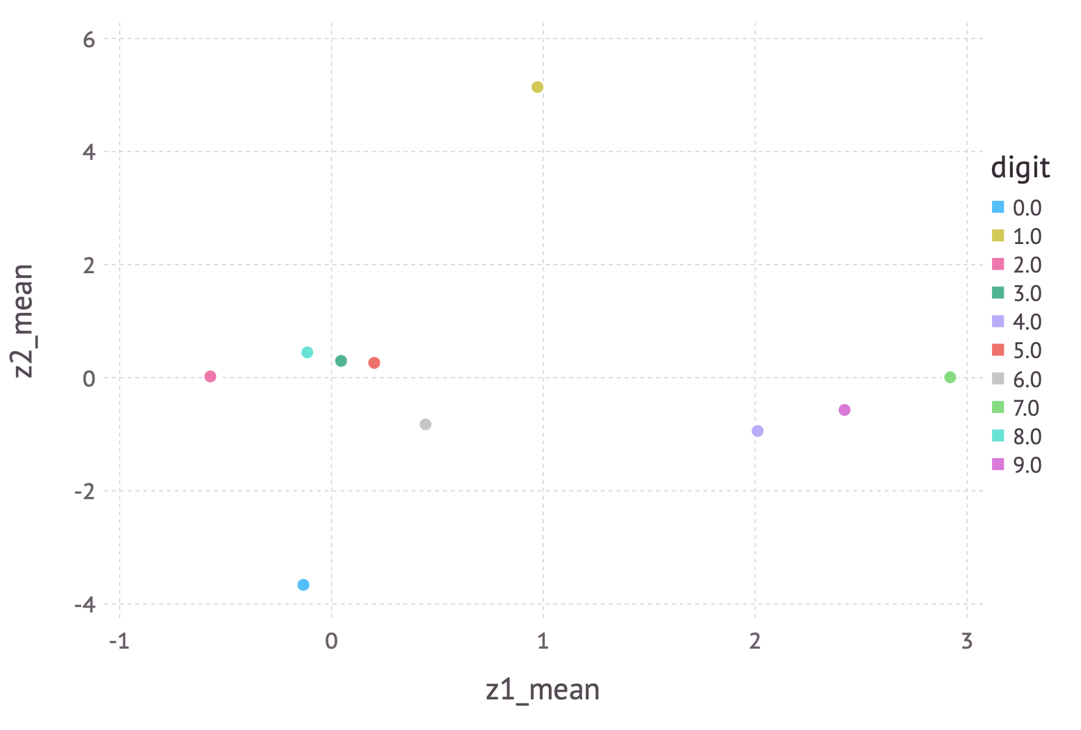
A few cute observations: (1) zero and one, which are highly distinct digits, are off in their own locations, far from everything else and each other, (2) four, seven, and nine are located close to each other, but far from everything else, and (3) three, five and eight are close together. All these observations make perfect sense when you look at the similarities between these digits.

Next, let’s look at the average reconstruction of each digit. That is, we take every digit in the dataset, pass it through the autoencoder and average the result across digits. We end up with something like this:

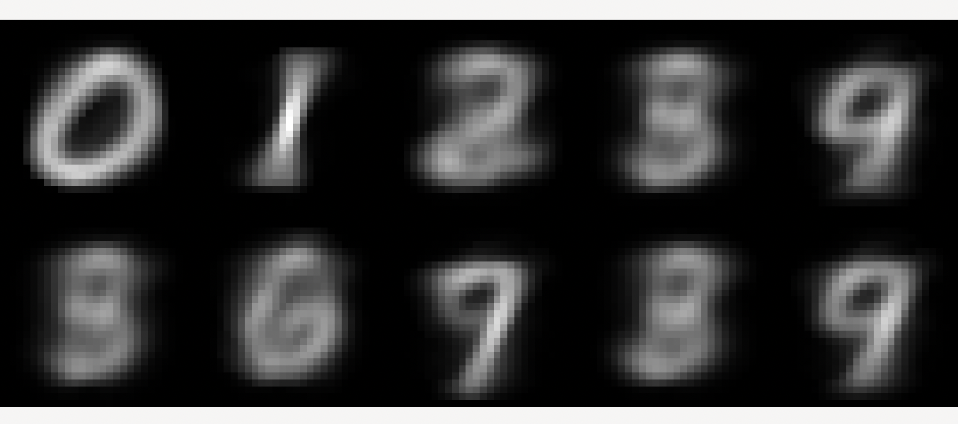
It’s far from perfect, but we’ve done an okay job! Every digit seems to be recognizably reconstructed on average. How can we improve our model? A good starting point is to replace the dense networks with convolutional networks.

Footnotes