Gaussian Processes
Given a sequence of points \(\mathbf{x}_1, \dots, \mathbf{x}_N\) in \(\mathbb{R}^K\), a Gaussian process \(f: \mathbf{x} \rightarrow \mathbb{R} \sim \mathcal{GP}(m, K)\) satisfies
\[\begin{align} \mathbf{f} &:= (f(\mathbf{x}_1), \dots, f(\mathbf{x}_N)) \sim \mathcal{N}(\mathbf{f} \ | \ \boldsymbol \mu, \boldsymbol \Sigma) \label{eq:gp} \\ \mu_i &= m(\mathbf{x}_i) \\ \Sigma_{i,j} &= K(\mathbf{x}_i, \mathbf{x}_j) \end{align}\]The idea is that the Gaussian process defines a prior over the function \(f\). However, it does not actually tell us how to sample \(f\) in its entirety. Instead, it tells us how to sample \(f\) point-wise. In particular, it says that any arbitrary sample of points is normally distributed. This a potentially high-dimensional distribution, as we can sample \(f\) at as many points as we wish. The key to the game is the assumption that the covariance is a function of \(\mathbf{x}\). Useful choices of the kernel, \(K\), will result in a high covariance between values of \(f\) sampled at points \(\mathbf{x}_i, \mathbf{x}_j\) that are close together, which results in a smoothly varying function. How smooth is determined by parameters of the kernel function.
A typical choice of kernel function is the radial basis function,
\[\begin{equation} \kappa(\mathbf{x}, \mathbf{x}^\prime) = \exp \left( -\frac{1}{2} (\mathbf{x} - \mathbf{x}^\prime)^{\top} \boldsymbol \Sigma^{-1}(\mathbf{x} - \mathbf{x}^\prime) \right) \end{equation}\]which describes a normal distribution centered at \(\mathbf{x}^\prime\) with variance \(\boldsymbol \Sigma\). But we are free to choose any kernel we wish so long as it results in positive-definite covariance matrix.
How can we use these things? Gaussian processes are used for non-parametric regression. They are non-parametric because we don’t specify a parametric form for the approxmation–only for the kernel function. They are typically used for spatial, temporal, or spatio-temporal regression: think of them as a method for curve fitting without having to specify the form of the curve. In some cases the function \(f\) is the primary object of interest; in other cases, \(f\) plays a supporting role in a larger probabilistic model.
Example A canonical example of Gaussian processes is given by the following regression problem. Suppose that we observe a time series \(y_i, \dots, y_N\) at corresponding times \(x_i, \dots, x_N\). We imagine that \(\mathbf{y}\) is a noisy observation of the process of interest, \(f(x)\), which we model as a Gaussian process. Thus, our model is
\[\begin{align} f &\sim \mathcal{GP}(f \ | \ 0, K) \\ y \ | \ f &\sim \mathcal{N}(y \ | \ f, \Sigma) \end{align}\]We want to learn about \(f\), so we do as any good Bayesian and consider it’s posterior distribution: \begin{align} f \ | \ y \propto \mathcal{N}(f, \Sigma) \times \mathcal{GP}(0, K) \end{align} Unfortunately, we have no idea what the righthand side of this equation even means: what is a normal distribution centered at the function \(f\), and how do I sample from \(\mathcal{GP}(0, K)\)? What we need to do instead is to consider a sample of this function, \(\mathbf{f} = (f_1, \dots, f_N)\), taken at the same moments that we observe \(\mathbf{y}\). Our assumption that \(f\) is generated by a Gaussian process tells us that any such sample is normally distributed. Now we can re-write the model as:
\[\begin{align} \mathbf{f} &\sim \mathcal{N}(\mathbf{f} \ | \ \mathbf{0}, \Sigma_f) \\ \mathbf{y} \ | \ \mathbf{f} &\sim \mathcal{N}(\mathbf{y} \ | \ \mathbf{f}, \Sigma_y), \end{align}\]which is a linear Gaussian system whose posterior is given by
\[\begin{align} p(\mathbf{f} \ | \ \mathbf{y}) &= \mathcal{N}(\mathbf{f} \ | \ \boldsymbol \mu_{f | y}, \boldsymbol \Sigma_{f | y}) \\ \boldsymbol \Sigma_{f | y}^{-1} &= \boldsymbol \Sigma_f^{-1} + \boldsymbol \Sigma_y^{-1} \\ \boldsymbol \mu_{f | y} &= \boldsymbol \Sigma_{f | y} \left[ \boldsymbol \Sigma_y^{-1} \mathbf{y} \right] \end{align}\]In case you are wondering, I did not recall this fact off the top of my head. Nor did I derive this posterior (although that is a good exercise): I simply knew that it is a well-known result for linear Gaussian systems, and therefore easy to look up. In summary, regression using Gaussian processes amounts to assuming a linear Gaussian system between the latent process \(\mathbf{f}\) and the observed process \(\mathbf{y}\), where the distribution of the former is determined by a the choice of kernel function \(K\).
Example As a somewhat more interesting example, consider the so-called log Gaussian Cox process (LGCP). This process is used to model the arrival of events whose likelihood varies over time, i.e., it is an inhomogeneous Poisson process. Specifically, we assume that the arrival of events follows as Poisson process whose intensity is determined by a Gaussian process:
\[\begin{align} f &\sim \mathcal{GP}(f \ | \ 0, K) \\ y &\sim \mathcal{PP}(y \ | \ \lambda(t) := \exp(f(t))) \end{align}\]Again, we cannot infer \(f\) directly, but must satisfy ourselves to consider a vector \(\mathbf{f}\) of observations at times \(x_1, \dots, x_N\). The posterior of this vector is given by
\[\begin{align} p(\mathbf{f} \ | \ y) \propto \mathcal{PP}(y \ | \ \boldsymbol \lambda) \times \mathcal{N}(\mathbf{f} \ | \ 0, \boldsymbol \Sigma) \end{align}\]In this case, we have no idea what the posterior distribution looks like. Thus, we will need to rely on sampling methods to approximate it. Neal, 2003 proposed a Metropolis-Hastings algorithm for sampling such distributions. The proposal distribution is given by
\[\begin{align} \mathbf{f}^\prime &= \sqrt{1 - \epsilon^2} \ \mathbf{f} + \epsilon \boldsymbol \nu \\ \boldsymbol \nu &\sim \mathcal{N}(\boldsymbol \nu \ | \ 0, \boldsymbol \Sigma) \end{align}\]with acceptance probability
\[\begin{equation} p(\text{accept}) = \min \left(1, \frac{p(y \ | \ \mathbf{f^\prime})}{p(y \ | \ \mathbf{f})} \right) \end{equation}\]In words, the proposal is a mixture of the current sample and a draw from the Gaussian process prior, which is always accepted if \(\mathbf{f}^\prime\) has a higher likelihood than \(\mathbf{f}\).
Murray et al., 2010 introduced an alternative method, ellpitical slice sampling, which eliminates the need to select the step size, \(\epsilon\). The name of this algorithm derives from its proposal,
\[\begin{equation} \mathbf{f}' = \mathbf{f} * \cos(\theta) + \boldsymbol \nu \sin(\theta) \end{equation}\]which describes an ellipse passing through \(\mathbf{f}'\) and \(\boldsymbol \nu\), combined with a “slice sampling” technique that adaptively adjusts \(\theta\).
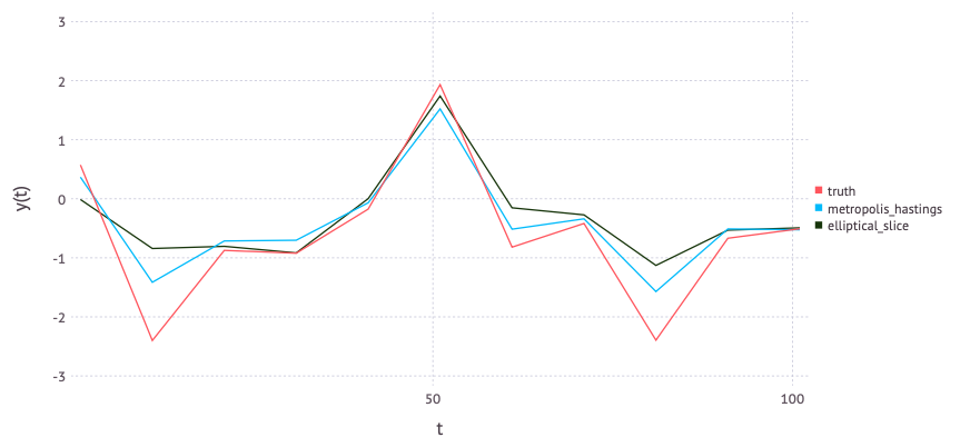 An example of sampling to estimate a log Gaussian Cox process. Time is shown along the \(x\)-axis and the (unobserved) Gaussian process is plotted on the \(y\)-axis. Curves represent the means of 100 draws from the sampling algorithm.
References
Neal, 2003 R. M. Neal. Slice sampling. Annals of Statistics, 31(3):705–767, 2003.
Murray, 2010 Iain Murray, Ryan Adams, and David MacKay. Elliptical slice sampling. In Proceedings of the Thirteenth International Conference on Artificial Intelligence and Statistics, volume 9, pages 541–548. PMLR, 13–15 May 2010.