Policies and Optimality
In the last lecture I introduced the general setting of deep reinforcement learning, which consists of computational agents interacting with a digital environment, earning rewards, and observing how its actions affect the future state of the world. Formally, this system is described as a Markov Decision Process. In this lecture I want to discuss how agents interact with their environment, describe how we evaluate the fitness of agents’ strategies, and finish by defining what is meant by “optimality” in reinforcement learning.
Policies
An agent’s actions are determined by a policy, which specifies the probability of every possible action that our agent can take in each state of the world. For simplicity, let’s assume that our world is finite so that we can enumerate the states of the world \(s_t \in \{0, 1, \dots, K - 1\} = \mathcal{S}\) as well as the possible actions \(a_t \in \{0, 1, \dots, N\} = \mathcal{A}\). For each action \(a \in \mathcal{A}\) and each state \(s \in \mathcal{S}\), a policy defines the probability our agent performs the action at time step \(t\):
\[\pi(a \ \vert \ s) = p(a_t = a\ \vert \ s_t = s)\]The policy defines a proper probability distribution, so we can use it to compute statistical quantities such as the expected reward at time \(t\):
\[\mathbb{E}_{\pi} \left[ r_t \ \vert \ s_t = s \right] = \sum_{a} \pi(a \ \vert \ s) \sum_{r_t, \ s_{t + 1}} p(r_t, s_{t + 1} \ \vert \ s_t = s, a_t = a) \ r_t\](The notation \(\mathbb{E}_{\pi}[x]\) is shorthand for \(\mathbb{E} \left[ x \ \vert \ a_t \sim \pi(a \ \vert \ s) \right]\). More generally, it means that every action is chosen according to \(\pi\)). If we follow a deterministic policy, then \(\pi\) collapses and we can instead think of it as a mapping from states to actions, \(\pi: \mathcal{S} \rightarrow \mathcal{A}\). In that case, the above expectation simplifies to
\[\mathbb{E}_{\pi} \left[ r_t \ \vert \ s_t = s \right] = \sum_{r_t, \ s_{t + 1}} p(r_t, s_{t + 1} \ \vert \ s_t = s, a_t = \pi(s_t)) \ r_t\]Our goal in reinforcement learning is learn optimal policies. You may be wondering why our policy doesn’t take time into account—why don’t we need to specify what action to perform at each time step? It turns out that framing the problem setting as a Markov Decision Process means that we don’t need to think in terms of policies that span multiple time steps: we only need to determine the best action to perform in each state of the world. Such policies can lead to sophisticated strategies because agents learn to move from “bad” states to “good” states.

Consider the following concrete example. Suppose we are training an agent to play the classic Atari game, Breakout. The optimal strategy in Breakout is essentially to make a hole along one side of the bricks, then hit the ball through the hole so that it bounces around endlessly on top of the bricks. As we normally describe it, the strategies seems to be intimately connected to time: first we do one thing (make the hole), then we do another (hit the ball through the hole). But we can equally describe this strategy in terms of states: if the world doesn’t have a hole, perform actions that make a hole, and if the world has a hole, perform actions that lead to the ball going through the hole. So really we just need to know which states we should move towards from whatever state we find ourselves in. This is how the reinforcement agent views the world.
Values
There are two important functions associated with every policy that we use to evaluate fitness, and which form the basis of reinforcement learning algorithms. The value of a policy is the expected return (sum of discounted rewards) “under the policy”,
\[V^{\pi}(s) = \mathbb{E}_{\pi} \left[ R_t \ \vert \ s_t = s \right] = \mathbb{E}_{\pi} \left[ \sum_{\tau=t}^{T} \gamma^{\tau - t} r_{\tau} \ \vert \ s_t = s \right],\]where the notation \(\mathbb{E}_{\pi}\left[ \dots \right]\) means that all actions are performed with the probabilities specificed by \(\pi\). Notice that the value of a policy depends on the current state: a policy might work well in one state of the world (high value), and poorly in another (low value). The goal of reinforcement learning is to choose the policy that has the highest value in all states of the world—more on this in a moment.
In addition to the value function, reinforcement learning relies heavily on the related concept known as an action-value function (also commonly referred to as the “Q-function”). The action-value function of a policy is its expected return assuming we perform an arbitrary action \(a\) at time step \(t\) and then follow the policy,
\[Q^{\pi}(s, a) = \mathbb{E}_{\pi} \left[ R_t \ \vert \ s_t = s, a_t = a \right].\]The only difference between the action-value function and the value function is the initial action performed: the value function follows the policy, while the action-value deviates from the policy. Action-value functions are useful because they allow us to ask the “what if” question (“What if I performed action \(X\) instead of action \(Y\)?”), which is obviously a useful question to consider if we’d like to improve our policy!
It’s worth pointing out (and you should convince yourself) that there is a simple relationship between the value and the action-value function:
\[V^{\pi}(s) = \mathbb{E}_{\pi} \left[ Q^{\pi}(s, a) \right],\]and
\[Q^{\pi}(s, a) = \mathbb{E}_{\pi} \left[ r_t + \gamma V^{\pi}(s_{t + 1}) \ \vert \ s_t = s, a_t = a \right].\]Optimality & The Bellman Equation
Clearly this value function is important—in some sense it is the only thing that matters (it’s what we’re trying optimize after all). But how do I calculate the value of a policy? Let’s consider a simplified problem where we can directly compute the value of a policy. So imagine that we are faced with a sequence of heads-or-tails decisions and that reward we receive depends in some arbitrary way on the sequence of coin flips we’ve seen so far. The situation is represented by a binary tree, where the value at each node represents the reward associated with the corresponding sequence of coin flips, as depicted below.
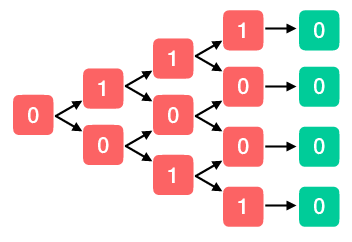
As shown, we flip the coin four times before the game ends. How do we decide what path to follow? The first step is to ask what the expected value of the game is after the second to last coin flip (the last columns of red nodes). The game ends on the next step no matter what, meaning that all states lead to the terminal state with no reward. So the expected reward at each node is the reward received at that node plus zero.
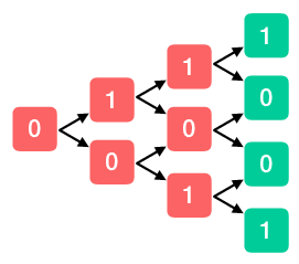
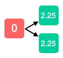
Now we repeat this analysis for the states following the second coin flip. We’ll fill in each of the expectations we just calculated (the new green nodes), and we can now ignore the terminal state. Our goal is to calculate the expected return from each node, which (if we are dealing with a fair coin) is equal to its reward plus the average of its childrens values. For example, the top node earns a reward of one, and the average of its children is one-half, so that node is overwritten by one and one-half.

We keep repeating this process until we arrive at the root node, at which point we have calculated the expected value of the policy.

This example motivates a straightforward method to compute the value of the policy: start from the end and work backwards. At the end of the game—at time \(T+1\)—the value is zero, so we can write \(V_{T + 1} = 0\). Now we take one step back and ask what the value is going forward. At time \(T\) we earn a random reward \(r_T\), then transtion to \(s_{\text{end}}\) and earn zero additional reward, so the value is \(V_T = \mathbb{E}_{\pi}\left[ r_T \right]\). Let’s continue to move backward in time: at time \(T - 1\) we earn a random reward \(r_{T-1}\), then we transition to state \(s_T\) where we already know that we will earn a value of \(\mathbb{E}_{\pi}\left[ r_{T} \right]\) going forward. Therefore the value at time \(T-1\) is \(\mathbb{E}_{\pi} \left[ r_{T-1} + \mathbb{E}_{\pi} \left[ r_T \right] \right] = \mathbb{E}_{\pi} \left[ r_{T - 1} + V_T \right].\)
If we continue moving backwards in this fashion we’ll see that every step along the way the value at step \(t\) is always equal to \(\mathbb{E}_{\pi} \left[ r_{t} + V_{t + 1} \right],\) which we can always compute because we started by saying that \(V_{T+1} = 0\). Thus, we have figured out a simple algorithm to compute the value of our random policy. The key was recursion: relate the value today to the value tomorrow. In this example we didn’t worry about states of the world, but essentially the same logic works in the Markov Decision Process setting of reinforcement learning. The Bellman equation demonstrates that the value of a given policy satisfies a particular recursive property:
\[V^{\pi}(s) = \mathbb{E}_{\pi} \left[r_t + \gamma V^{\pi}(s_{t + 1}) \ \vert \ s_t = s \right]\]In words, the expected value of following a policy can be broken into the expected reward that period and the expected return from all subsequent periods, and the later is simply the value one period in the future. We need to take the expectation of the future value because the future state is random, and where we end up next period depends on the action we choose today through the transition probability \(p(r_{t + 1}, s_{t + 1} \ \vert \ s_t, a_t)\).
The Bellman equation is interesting because it defines \(V^{\pi}\) in the sense that the value function of \(\pi\) is its unique solution. Just as in the example above, the Bellman equation tells us how to compute the value of a policy. In fact, if there are a finite number of states—let’s say \(K\) to be concrete—then the Bellman equation is really a \(K \times K\) system of equations, and \(V^{\pi} \in \mathbb{R}^K\) is its solution, which you can perhaps see this more clearly by writing out the Bellman equation using probabilities:
\[V^{\pi}(s) = \sum_a \pi(a \ \vert \ s) \sum_{r_t, \ s_{t + 1}} p(r_t, s_{t + 1} \ \vert \ s_t = s, a_t = a) \left[ r_t + \gamma V^{\pi}(s_{t + 1}) \right]\]This equation holds for every \(s \in \mathcal{S}\), and so for each state we get an equation that involves known probabilities (\(\pi\) and \(p\)) and the value in each state \(s_{t + 1} \in \mathcal{S}\).
Now the goal of reinforcement learning is to learn optimal policies (or approximately optimal policies). So how do we define an optimal policy? A policy is optimal if its value is at least as large as any other policy in every state of the world. It’s common to denote an optimal policy (which may not be unique) by \(\pi^{\ast}\), and to denote the corresponding value and action-value functions by \(V^{\ast}\) and \(Q^{\ast}\). While the optimal policy may not be unique, the optimal value function is, with the practical implication that it isn’t necessary to directly look for the optimal policy. Instead, we can look for the optimal value, and then define an optimal policy based on the optimal value function (more of this in the following lecture).
Whatever the optimal value is, it must adhere to the Bellman equation (it is the result of some policy after all). However, the optimality of the policy allows us to write this equation out slightly differently:
\[V^{\ast}(s) = \max_a \mathbb{E}_{\pi^\ast} \left[ r_t + \gamma V^{\ast}(s_{t + 1}) \ \vert \ s_t = s, a_t = a \right]\]Writing out the “\(\max_a\)” doesn’t really change this expression from what we wrote down before because (by definition) following \(\pi^{\ast}\) already implies that we take a maximizing action, but the notation makes it explicit that we only need to worry about what happens from this period to the next. The Bellman equation is at the core of many deep reinforcement learning algorithms. In my next post, I’ll take a look at the role it plays in some classical reinforcement learning algorithms.
References
- [SB] Sutton & Barro,. Reinforcement Learning: An Introduction, (2018).