Introduction to Deep Reinforcement Learning

Monday, July 8, 2019

This is the first in a series of introductory lectures on deep reinforcement learning. I plan to follow the classic text by Sutton and Barro [SB], but I will also borrow from the lecture notes used in Sergey Levine’s course on deep reinforcement learning taught at Berkeley for the last few years. We won’t get into the “deep” part of “deep reinforcement learning” for a few lectures, but hopefully laying out some groundwork will make the more modern ideas to come more meaningful.

The Goal of Reinforcement Learning

The goal of reinforcement learning is to train computers to perform complex, dynamic tasks, which generally involve planning. From a mathematical perspective, reinforcement learning presents itself as a computational—at times almost heuristic—alternative to traditional control theory. Both fields offer solutions to the general problem of determining an optimal course of action in a dynamic, and possibly uncertain, environment, which I refer to as the “control problem”. Control problems are complicated, but we can break them down into two parts. First, there is a time series or stochastic processes component, which reflects how the system changes over time as well as how the system reacts to actions performed by the agent. Second, there is an optimization component, which involves determining how to act to alter—or control—these dynamics so that the system achieves some desired outcome, or follows some optimal trajectory.

Traditional mathematical approaches to these types of problems represent some of the crowning achievements of applied mathematics. In some cases, they provide exact formulae describing what actions to take and when; for a surprisingly board range of problems, they prove that certain numerical methods generate approximate solutions that can be made arbitrarily close a ground truth solution. To give just one example, the “genius” of modern finance—the “astrophysics” that is derivatives pricing—is nothing more than applied stochastic control. But for all the beauty of mathematical optimal control, it doesn’t have the flexibility required to solve many apparently simple real-world problems. The real world is messy, and it is in that messy world that reinforcement learning takes center stage.

The control problem

Agents & Environments

Reinforcement learning revolves around agents and environments. An agent is a computer that makes decisions and selects actions to perform; an environment is the world that the agent observes and interacts with. Reinforcement learning generally considers sequences of decisions made over time, and problems in which the actions an agent selects at one time step affect the environment the agent observes in the following step. In principle, these are just optimization problems, but they are more complicated than “standard” optimization problems because they require the agent to determine the optimal action to perform in every possible state of the world.

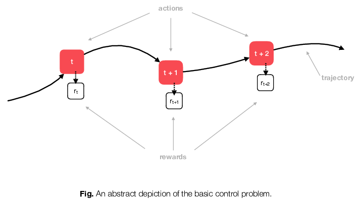
Unlike classic mathematical approaches, reinforcement learning algorithms involve interaction between the agent and the environment. Agents learn about the environment by performing actions and seeing how the environment evolves, as depicted in the figure above. At each point in time, the agent looks at the current state of the world (or her perception of it at least), selects an action to perform, and then observes both a reward as well as the next state of the world. In other words, we design reinforcement learning agents to learn through experimentation, through trial-and-error.

One of the fundamental problems that arises in reinforcement learning is the trade-off between exploitation and exploration. Whenever an agent performs an action, it affects both the reward received and the next state of the world. One the hand, the agent wants to select actions that it believes generate higher rewards (because its trying to maximize rewards). On the other hand, if it only chooses actions that it currently believes to generate higher rewards, it might never learn other actions that lead to states of the world where she can generate even higher rewards. It is a situation that we are all familiar with: do we go with the best option that we know, or do we take a chance and try something new? Our choice will determine our information set (we’ll never know if we should have taken that other job offer), and therefore what we can learn—and likewise for our agent.

I’ve been talking about “time” and “states”. It’s worth pointing out that “time” in this context doesn’t mean “natural time”: it’s just an ordering of events, which can have an arbitrary amount of (natural) time between them. For example, time might count each occurrence of a user visiting a web application, in which case the steps will be spaced out randomly. Alternatively, we might be thinking about an agent that checks the state of the world on a fixed schedule (e.g. once per second). The goal of reinforcement learning is not to model or predict the timing of events, but to determine how to respond to events as they occur. Likewise, “state” should not be construed to mean a “natural state” of the world, but can be thought of abstractly. State can mean measurable quantities like location and speed, but it can also refer to a “state of mind” or a “state of thought” [SB].

Dynamics

The theory of reinforcement learning centers on a simple but flexible assumption regarding the way the environment works: we assume that whatever happens each time step depends only on the current state of the world and on the agent’s present choice of action. The rest of history is irrelevant to what happens this time step. In other words, it doesn’t matter how we arrived at a state, it only matters that we are in that state.

Mathematically, we call the system a Markov decision process (MDP). Let’s denote the state of world at time \(t\) by \(s_t\), our agent’s action by \(a_t\), the rewards received by \(r_t\), and the new state \(s_{t + 1}\). The Markov assumption says that \(r_t\) and \(s_{t + 1}\) are determined by some probability distribution represented by some joint probability density

\[p(r_t, s_{t + 1} \ \vert \ a_t, s_t),\]

which completely describes the dynamics of the system—\(p\) is all we need to know in order to understand how the environment works. But we haven’t said anything about the nature of \(p\) other than that it is a valid probability distribution. In many applications, \(p\) is in fact a deterministic—but extremely complicated—function. Nonetheless, the assumption means that if it knows \(p\), then our agent can make optimal decisions based on the current state of the world, and nothing else.

mdp

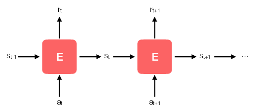
The figure above shows a canonical representation of the MDP. If you’ve studied recurrent neural networks, this diagram ought to look familiar—at a high level it’s the same as a vanilla RNN. Alternatively, you might see this figure as a special form of hidden Markov model in which we add an additional “forcing” variable \(a_t\) to the mix. Either way, the Markov assumption reduces the problem of understanding the dynamics of the system to that of learning a single distribution represented by \(p\). In the case of a hidden Markov model, \(p\) is typically a separable function taking the form \(p(r, s' \ \vert \ s, a) = f(r \ \vert \ s, a) \ g(s' \ \vert \ s, a)\). In the case of vanilla RNN, \(p\) is also separable, but \(f\) and \(g\) are represented by hidden layers instead of explicit probability distributions. In reinforcement learning we make no such assumptions about \(p\). As you will see, reinforcement learning often avoids learning about \(p\) directly.

It might seem to you that the Markov assumption is too restrictive: surely many interesting problems require us to know more than just the most recent history! In practice this isn’t really an issue because we are always free to redefine what we mean by “state”. For example, if you tell me that tomorrow’s weather depends on the last two days of weather, and not just yesterday’s weather, then I will simply change my definition of state from “the last day’s weather” to “the last two days’ weather”. As [SB] puts it, “This is best viewed a [sic] restriction not on the decision process, but on the state.” In other words, any process that we have a reasonable hope of controlling will satisfy the Markov property for some definition of the state.

Rewards

Agents learn optimal plans via reward signals designed and specified by us, their human overlords. Rewards can be understood by analogy with neurotransmitters (e.g. dopamine), which signal the desirability of different outcomes to the brain. Such neurotransmitters motivate us to perform actions that lead to (or avoid) particular states of the world through experience. In the case of reinforcement learning, researchers specify the amount of reward associated with the environment, and rewards are therefore arbitrary in some sense. On the other hand, the performance of a reinforcement learning algorithm is highly dependent on the choice of rewards, with poorly chosen rewards resulting in agents that fail to learn desired outcomes, or grow “addicted” to sub-optimal behaviors.

Fortunately, a natural choice for rewards will often work. For example, an agent trained to play a two-player video game might earn a reward of one for winning, and negative one for losing, or it might earn rewards proportional to its score in a one-person game. In other cases an appropriate reward system might be less obvious: what rewards should we specify for a robot learning to walk? The key to remember is that agents generally have little pre-programmed “knowledge”: unlike the natural world, they lack genetic predisposition towards particular behaviors and will engage in any manner of outrageous behavior if it elicits reward.

From the agent’s perspective rewards are just some numerical value; reinforcement learning algorithms encourage the computer to select actions that generate greater amounts of reward. In the typical reinforcement learning setting the agent’s goal is to maximize the expected amount of total reward received:

\[\max_{\{a_0, \dots, a_T\}} \mathbb{E} \left[ R \right] = \max_{\{a_0, \dots, a_T\}} \mathbb{E} \left[ \sum_{t = 0}^T \gamma^t r_t \right].\]

We refer to the quantity \(R\) as the return, and the expectation is taken with respect to the transition probability \(p(r_t, s_{t + 1} \ \vert \ a_t, s_t)\). The quantity \(\gamma\) is called the “discount factor”, and it imparts the agent with a time-preference over rewards: when \(\gamma < 1\), the agent prefers to receive rewards early rather than later, all else being equal.

It’s important to recognize that there is no aspect of risk in the above objective. From a behavioral perspective, its clear that individuals’ actions will generally reflect both risk and reward. For this reason economists typically assume that agents choose actions that maximize a so-called utility function, \(U\), which involves both the expectation and variance (or standard deviation) of rewards. For example, an investor might seek to maximize

\[U(R) = \frac{\mathbb{E}\left[ R \right]}{\text{var} \left[ R \right]},\]

reflecting the intuitive notion that for any fixed expected return, a lower risk outcome is preferable. This is a interesting topic because adjusting for risk tolerance is likely essential to making deep reinforcement learning solutions palatable in many practical settings.

Reward design deserves more attention that I can give it here, but I feel it’s important to reiterate [SB], who point out that rewards are not a good mechanism for encouraging solutions with certain properties. We don’t use rewards to encourage a robot to learn sub-tasks because the agent might learn to only perform the sub-tasks, ignoring the outcome we actually care about! In other words, we want to focus agents on one goal, and let the agent figure out how to achieve that goal.

Infinite vs Finite Horizon

Textbook presentations of reinforcement learning make a point of distinguishing between problems which eventually come to a finish—“finite horizon problems”—and problems that continue indefinitely with non-zero probability, so-called “infinite horizon problems”. The distinction has theoretical implications, but I view it as largely a distraction. One reason that the infinite horizon case is brought up is to motivate the idea of the discount factor mentioned above, which is optional in the finite horizon case, but required in the infinite horizon case to guarantee that \(R\) is well-defined.

As mentioned above, there is (potentially) a strong behavioral motivation behind discount factors in either case, but the most successful applications of deep reinforcement learning thus far have come in settings where time-preference over rewards plays an minor role (think \(\gamma \approx 0.99\)). Nonetheless, if a reinforcement learning agent is used to learn an economic task, choosing an appropriate discount factor might be critical to finding an acceptable solution.

Examples

Let’s take a brief look at three example environments. While admittedly contrived, these examples are useful for testing algorithms and simple to understand. Each of these examples is available in OpenAI’s gym package.

CartPole

The pole-balancing problem is a classic in reinforcement learning. The environment consists of a cart that moves side-to-side along on a one-dimensional track, with a long pole attached to the cart via a hinge. When the cart is pushed one way, the pole falls in the opposite direction. We start the environment by placing the pole is some random “not-quite-vertical” position, and the goal of the agent is to keep the pole from falling over (or not letting the pole fall past a certain angle, after which it is impossible to bring the pole back upright).

The only information that the agent needs to know is the position of the cart, \(x_t\), and the angle of the pole, \(\theta_t\). Therefore the state is two-dimensional: \(s_t = (x_t, \theta_t).\) There are two available actions: “push left”, and “push right” (assume that the agent can only push with some fixed amount of force). We say that the state space is continuous, while the action space is discrete. You could make the problem more complicated by allowing the agent to choose the direction to push and the amount of force to use. In that case, the action space would be mixed, the direction being discrete, and the force continuous.

The gym package’s implementation of the pole-balancing problem is called CartPole (shown above). The environment is extremely simple to solve. We don’t need any fancy algorithms to solve it, but it is useful for debugging: if it doesn’t solve CartPole, it doesn’t work. I also like to think of the inverse statement as being almost true: if it solves CartPole, it probably works—so if you’re having problems with some other environment, maybe focus on errors in the environment-specific part of your code.

LunarLander

A classic problem in optimal control considers how to land a rocket on the moon. The goal is actually to land the rocket using the minimal amount of fuel (as otherwise you could always make a pillow-soft landing by burning through as much fuel as you want). Landing the rocket means that you arrive at a specific location (or within a specified region) with zero velocity and zero acceleration (and you don’t crash). In a standard version of this problem—which can be solved analytically [E]—the rocket drops straight down under the influence of gravity alone, and the pilot/onboard computer only needs to determine how much upward thrust to provide. In that case, the state space is continuous and one-dimensional (\(y_t =\) height), as is the action space (\(a_t =\) thrust).

The gym version of this problem is a bit more interesting. First, the lander is dropped with a random orientation, so that every episode begins in a random state. Second, the lander is equipped with left-oriented and right-oriented thrusters in addition to a bottom thruster. The agent can only fire one of the thrusters (or none) at any instant, and the thrusters only have one setting (“full blast”). The state is described by eight variables:

x_position
y_position
x_velocity
y_velocity
angle
angular_velocity
left_leg_contact
right_leg_contact

The first six variables are continuous, while the last two are discrete (they just indicate whether the legs are on the ground or not).

Solving this environment is more difficult than solving the CartPole environment, but still simple enough that it can serve as a useful testing ground for rapid prototyping of new algorithms. It doesn’t require any special handling of the observations, and if the algorithm works, it will converge relatively quickly.

Pong

Dominating video games is the application of reinforcement learning that has received a lot of attention in the last few years. Pong is one of the easiest/fastest video games to learn. Reinforcement learning researchers use Atari games as benchmarks in research because they offer a wide range of tasks (from Pong to Seaquest), and because packages like OpenAi provide a standardized platform for training new algorithms against the full range of tasks. Computer agents learn to play Pong using essentially the same information that human players have access to: a “visual” representation of the game provided as a matrix of pixels. Agents are allowed perform any of the actions that a human can take. In Pong, this means “do nothing” (also referred to as “NOOP” for “No Operation”), “move paddle up”, or “move paddle down”.

The following snippet of code demonstrates how to run a random policy on Pong for one episode with gym:

import gym
env = gym.make('Pong-v4')
env.reset()
while True:
    state, reward, done, info  = env.step(env.action_space.sample())
    if done:
        break

This seems like a good place to stop for now. In the next lecture we’ll discuss policies and optimality.

References

[SB] Sutton & Barro,. Reinforcement Learning: An Introduction, (2018).
[E] Evans. “An Introduction to Mathematical Optimal Control theory”, (1983).